
F 3 GEOGRAPHY
STATISTICS
COMPOUND/CUMULATIVE/DIVIDED
BAR GRAPH
Major cash crops exported in Kenya in tonnes
| CROP | 1990 | 1991 | 1992 | 1993 | 1994 |
|---|---|---|---|---|---|
| COFFEE | 4500 | 5000 | 5200 | 6000 | 5900 |
| TEA | 1300 | 1100 | 2500 | 2100 | 2200 |
| MAIZE | 800 | 900 | 500 | 400 | 400 |
| WHEAT | 600 | 500 | 600 | 700 | 500 |
Steps
| CROP | 1990 | CT | 1991 | CT | 1992 | CT | 1993 | CT | 1994 |
|---|---|---|---|---|---|---|---|---|---|
| COFFEE | 4500 | 4500 | 5000 | 9500 | 5200 | 14700 | 6000 | 20700 | 5900 |
| TEA | 1300 | 5800 | 1100 | 6900 | 2500 | 9400 | 2100 | 11500 | 2200 |
| MAIZE | 800 | 6600 | 900 | 7500 | 500 | 8200 | 400 | 8600 | 400 |
| WHEAT | 600 | 7200 | 500 | 7700 | 600 | 8800 | 700 | 9500 | 500 |
| TOTAL | 7200 | 7500 | 8800 | 9200 | 9000 | ||||
- Set cumulative totals for the data each year.
- Draw vertical axis (Y) to represent the dependent variable.
- Draw horizontal axis (X) to represent the independent variable.
- Label both axes using a suitable scale.
- Plot the cumulative values for each year.
- Use values for components to subdivide the cumulative bar.
- The subdivisions are placed in descending order with the longest at the bottom (coffee).
- Shade each component differently.
- Put title and key.
Advantages
- It is easy to construct.
- It has a good visual impression.
- There is easy comparison for the same component in different bars because of uniform shading.
- Easy to interpret because bars are shaded differently.
- Total value of the bar can be identified easily.
Disadvantages
- It doesn’t show the trend of components (change over time).
- Cannot be used to show many components as there is limited space upwards.
- Tedious as there is a lot of calculation work involved.
- Not easy to trace individual contribution made by members of the same bar.
- Poor choice of vertical scale causes exaggeration of bars’ length leading to wrong conclusions.

Analysis
- Coffee was the leading export earner in the five years.
- Tea was the second leading export earner.
- Wheat had the lowest export quantity.
- 1993 recorded the highest export quantity.
- 1990 recorded the lowest export quantity.
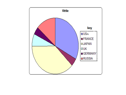
PIE CHART / DIVIDED CIRCLES / CIRCLE CHARTS
- A circle subdivided into degrees used to represent statistical data where component values have been converted into degrees.
Major countries producing commercial vehicles in the world in 000s
| USA | FRANCE | JAPAN | UK | GERMANY | RUSSIA |
|---|---|---|---|---|---|
| 1800 | 240 | 2050 | 400 | 240 | 750 |
Steps
- Convert components into degrees.
USA: 1800 × 360 / 5480 = 118.2°
FRANCE: 240 × 360 / 5480 = 15.8°
JAPAN: 2050 × 360 / 5480 = 134.7°
UK: 400 × 360 / 5480 = 26.3°
GERMANY: 240 × 360 / 5480 = 15.8°
RUSSIA: 750 × 360 / 5480 = 49.3°
- Draw a circle of convenient size using a pair of compasses.
- From the centre of the circle, mark out each calculated angle using a protractor.
- Shade the sectors differently and provide the key for various shadings.
Advantages
- Gives a good, clear visual impression.
- Easy to draw.
- Can be used to present varying types of data, e.g., minerals, population, etc.
- Easy to read and interpret as segments are arranged in descending order and are well shaded.
- Easy to compare individual segments.
Disadvantages
- Difficult to interpret if segments are many.
- Tedious due to a lot of mathematical calculations and marking out of angles involved.
- Can’t be used to show trend/change over a certain period.
- Small quantities or decimals may not be easily represented.
Analysis
- The main producer of commercial vehicles is Japan.
- The second largest producer is USA followed by Russia.
- The lowest producers were France and West Germany.
PROPORTIONAL CIRCLES
This is the use of circles of various sizes to represent different sets of statistical data.
Table showing mineral production in Kenya from year 1998-2000
| MINERALS | QUANTITY IN TONNES | ||
|---|---|---|---|
| 1998 | 1999 | 2000 | |
| Graphite | 200 | 490 | 930 |
| Fluorspar | 30 | 255 | 450 |
| Soda ash | 270 | 300 | 350 |
| Diamond | 500 | 870 | 1270 |
| TOTAL | 1000 | 1915 | 3000 |
Steps
- Determine the radii of circles by finding the square roots of the totals:
1998: √1000 = 31.62 ≈ 32
1999: √1915 = 43.76 ≈ 44
2000: √3000 = 54.77 ≈ 55
- Scale: 1 cm represents 10 tonnes
1998 = 3.2 cm
1999 = 4.4 cm
2000 = 5.5 cm
- Using a pair of compasses, draw circles of different radii representing mineral production in Kenya between 1998 and 2000.
- Convert component values into degrees:
Component value / total value of data × 360
1998:
Graphite – 200 / 1000 × 360 = 72°
Fluorspar – 30 / 1000 × 360 = 10.8°
Soda ash – 270 / 1000 × 360 = 97.2°
Diamond – 500 / 1000 × 360 = 180°1999:
Graphite – 490 / 1915 × 360 = 92.1°
Fluorspar – 255 / 1915 × 360 = 47.9°
Soda ash – 300 / 1915 × 360 = 56.4°
Diamond – 870 / 1915 × 360 = 163.6°2000:
Graphite – 930 / 3000 × 360 = 111.6°
Fluorspar – 450 / 3000 × 360 = 54°
Soda ash – 350 / 3000 × 360 = 42°
Diamond – 1270 / 3000 × 360 = 152.3° - On the proportional circle for each year, use a protractor and mark out the angles.
- Shade the segments and then provide a key.
Advantages
- They give a good visual impression.
- Easy to compare various components.
- Simple to construct.
- Easy to interpret as segments are arranged in descending order.
- Can be used to present varying types of data.
Disadvantages
- Tedious in calculation and measurement of angles.
- Actual values represented by each component cannot be known at a glance.
- Difficult to accurately measure and draw sectors whose values are too small.
- Comparison can be difficult if the circles represent values which are almost equal.
Analysis/Conclusions
- Diamond was leading in production.
- The second leading mineral in production was graphite.
- The mineral with the lowest production was fluorspar.
NB: Revision questions assignment to be given.
Best end year regards, Merry X-mas By Mr H. Geog Dept Ibubi 2014
MAP WORK
Description of Relief
- Describe the general appearance of the entire area, e.g., hilly, mountainous, plain, undulating landscape, has many hills, isolated hills, etc.
- State the highest and lowest parts of the area.
- Look out for valleys which are occupied by rivers.
- Divide into relief regions such as plateau, escarpment, and lowland.
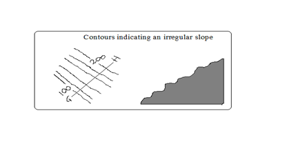
- Explain the type of slope, e.g., gentle, steep, even, or irregular.
- Direction of slope.
- Identify the landforms present in the area.
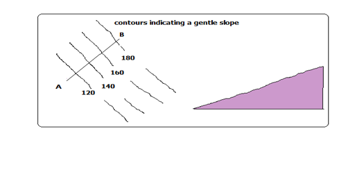
Gentle Slope
Slope is the gradient of land surface.
Gentle slope is one in which land doesn’t rise or fall steeply.
Contours are wide apart.
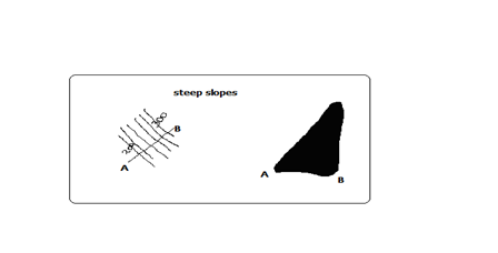
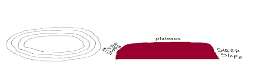
Steep Slopes
- Where land rises or falls sharply.
- Contours are close to each other.
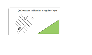
Even Slopes
- Shown by contours which are evenly spaced.
Uneven Slopes
- Indicated by unevenly spaced contours.
Convex Slopes
- One curved outwards.
- Indicated by contours which are close together at the bottom and widely spaced at the top.

Concave Slopes
- One curved inwards.
- Contours are close together at the top and widely spaced at the bottom.

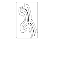
A Valley
- A low area between higher grounds.
- Indicated by U-shaped contours pointing towards a higher ground.

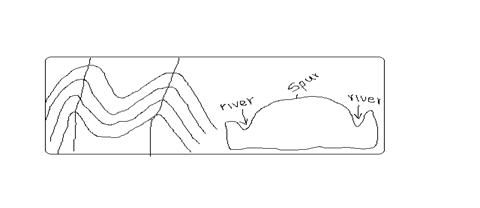
A Spur
- Land which is projected from high to low ground.
- Indicated by U-shaped contours bulging towards lower ground.
Interlocking Spurs
- Spurs which appear as if to fit together.
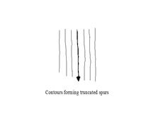
Truncated Spurs
- Spurs in glaciated highlands whose tips have been eroded and straightened.
Conical Hills
- Hills are uplands which rise above relatively lower ground.
- Conical hills are small rounded hills.

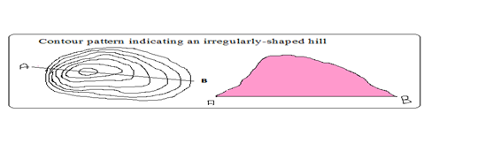
Irregular Shaped Hills
A hill with some sides with uneven gentle and others with uneven steep slopes.
Ridges
- A range of hills with steep slopes on all sides.
- A ridge can contain hills, cols, passes, or watershed.

A Col
- A low area which occurs between two hills.
A Pass
- A narrow steep-sided gap in a highland.
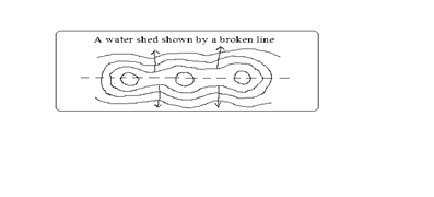
A Watershed
- The boundary separating drainage systems which drain in different directions.
- Escarpments and ridges often form watersheds.
Escarpment
- A relatively continuous line of steep slopes facing the same direction.
- Has two slopes: a long gentle slope (dip slope) and a short steep slope (scarp slope).

A Plateau
- A high flat land bound by steep slopes.
Description of Vegetation
Natural vegetation is classified as woodlands, thickets, scrubs, or grasslands.
Symbols are given as pictures of vegetation.
- Types present
- Distribution
- Reasons for distribution, e.g., seasonal streams, scrub or grassland due to low rainfall.
- Forests
Likely indications of the following in the area:
- Heavy rainfall
- Fertile soil
- Cool temperature depending on altitude
- Thickets and shrubs
- Seasonal rainfall
- Poor soil
- High temperature
- Riverine trees
- High moisture content in the river valley
Describing Drainage
- Identify drainage features present.
Natural drainage features include lakes, rivers, swamps, sea, rapids, waterfalls, cataracts, springs, deltas, fjords, sand or mud, and bays.
Artificial features include ponds, wells, boreholes, water holes, cattle dips, cattle troughs, canals, reservoirs, irrigation channels, aqueducts, water treatment plants, and man-made lakes.
- Identify main rivers by name.
- Size of rivers – big or small – shown by thickness of blue lines.
- Give the general direction of flow.
- Location of watershed if any.
- Characteristics of each feature.
a) Permanent Rivers
- Which flow throughout the year.
- Shown by continuous blue lines.

Likely indication of:
- Heavy rainfall
- Impermeable rocks
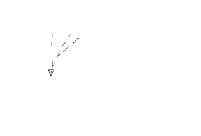
b) Seasonal Rivers
- Which flow seasonally or during the rain season.
- Shown by broken blue lines.
Likely indication of:
- Low rainfall
- River doesn’t have a rich catchment area
c) Disappearing Rivers
Blue lines ending abruptly.
Likely indication of:
- Permeable rocks
- Very low rainfall
- Underground drainage
- Identify drainage patterns and description.
Drainage pattern is the layout of a river and its tributaries on the landscape.
a) Dendritic
Resembles a tree trunk and branches or veins of a leaf.
Tributaries join the main river at acute angles.

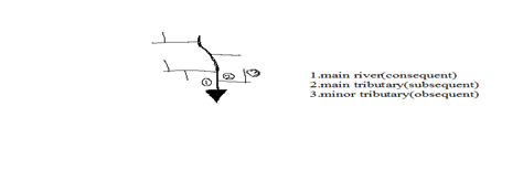
b) Trellis
Tributaries join the main river and other tributaries at right angles.
Common in folded areas where rivers flow downwards separated by vertical uplands.
c) Rectangular Pattern
Looks like a large block of rectangles.
Tributaries tend to take sharp angular bends along their course.

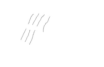
d) Parallel Pattern
Rivers and tributaries flow virtually parallel to each other.
Influenced by slope.
Common on slopes of high mountain ranges.

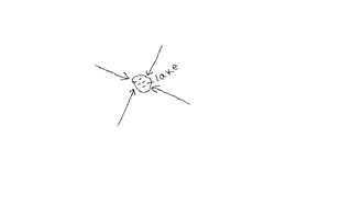
e) Centripetal Pattern
Rivers flow from many directions into a central depression such as a lake, sea, or swamp.
Examples are rivers flowing into some of the Rift Valley lakes such as Nakuru and Bogoria.
f) Annular Pattern
Streams (rivers which are small in size) are arranged in series of curves about a basin or crater.
It’s controlled by the slope.
g) Radial
Resembles the spikes of a bicycle.
Formed by rivers which flow downwards from a central point in all directions such as on a volcanic cone e.g., on Mt. Kenya, Elgon, and Kilimanjaro.

h) Fault-Guided Pattern
- Flow of river is guided by direction of fault lines.

Human/Economic Activities
Description of Human Activities
- Identify types.
- Evidence – man-made features.
- Reasons e.g., tea – cool temperatures and heavy rainfall.
Agriculture
a) Plantation farming
Evidenced by presence of:
“C” – coffee
Named estates e.g., Kaimosi tea estate
b) Small scale crop farming
- Cotton ginnery or sheds
- Coffee hulleries
- Posho mills for maize, millet, sorghum
- Tea factory/store
Livestock Farming
- Dairy farms
- Veterinary stations
- Cattle dips
- Creameries
- Water holes
- Dams
- Butcheries
- Slaughter houses
Mining
- Symbol for a mine/mineral works
- Name of the mine
- Particular mineral e.g., soda ash
- Quarry symbol
- Processing plant of a mineral e.g., cement indicates cement is mined in that area
Forestry/Lumbering
- Saw mills
- Forest reserves
- Forest station
- Forest guard post
- Roads ending abruptly into a forest estate used to transport logs to saw mills
Fishing
- Fish traps
- Fishing co-operative society
- Fish ponds
- Fish hatcheries
- Fisheries department
- Fish landing grounds (banda)
Manufacturing/Processing Industry
- Saw mills for lumber products
- Ginnery for cotton processing
- Mill for maize, millet, wheat processing
- Creameries for milk processing
- Factory for manufacturing or processing a known commodity
Services
a) Trade
- Shops
- Markets
- Stores
- Trading centres
b) Transport
i) Land
- Roads
- All weather roads – which are used all year round i.e., tarmac and murram roads.
- Dry weather roads – which are used reliably during dry seasons.
- Motorable tracks – rough roads which are used by people on foot and by vehicles in dry seasons.
- Other tracks and footpaths
- Railways, station, sidings, level crossing lines, and railway lights
ii) Air
- Airfields
- Airports
- Air strips
iii) Water
- Ferries
- Bridges
c) Communication
- Post offices (P.O.)
- Telegraph (T.G.)
- Telephone lines (T)
d) Tourism
- Camping sites
- Tourist class hotels and restaurants
- National parks
- Game reserves
- Curio shops
- Museums
- Historical monuments
e) Administration
- DO, DC, PC, police post, chiefs camp.
Social Services
a) Religious Services
- Church
- Mosque
- Temples
b) Education
- Schools
- Colleges
- Universities
c) Health Services
- Hospitals
- Dispensaries
d) Recreational Services
- Golf clubs/courses
- Stadiums
Description of Settlement
A settlement is a place with housing units where people live together.
- Densely distributed settlements – high concentration of settlements (black dots).
- Moderately distributed settlements – settlements moderate in quantity.
- Sparsely distributed settlements – few settlements spread over a large area.
- Very sparse if very few.
- Identify type of settlement patterns present.
- Type of Settlements.
a) Rural settlements
Consist of villages and homesteads in which people are involved in subsistence agriculture and traditional activities such as pottery, weaving, carving, etc.
b) Urban settlement
Consist of dense permanent and sometimes high buildings and population engaged in non-agricultural activities such as industrial activities.
Factors Influencing Settlement
1. Physical Factors
a) Climate
Areas with moderate temperatures and adequate rainfall are densely settled while those with extremely low or high temperatures have fewer settlements.
b) Relief
Terrain: Steep slopes are less settled due to thin soils and difficulty to erect buildings.
Aspect: Slopes facing away from the sun in high latitudes are less settled than those facing the sun.
Windward slopes of mountains on the path of rain-bearing winds are more settled due to heavy rainfall making them ideal for agriculture.
c) Drainage
Rivers and springs attract settlements because they provide clean water.
Areas with drainage swamps are less settled because it’s difficult to erect buildings and they also harbour mosquitoes and snails which cause diseases.
d) Vegetation
Dense forests discourage settlements because of wild animals and also harbour disease vectors such as tsetse flies e.g., Miombo woodland of Tanzania and Lambwe valley in Kenya.
e) Pests and diseases
Areas prone to pests and diseases are less settled because people like to live in healthy environments.
f) Natural resources
Settlements start where there is mineral extraction e.g., Magadi.
Lakes with abundant fish may also attract settlement.
g) Human Factors
i) Political factors
- 1967 Tanzania settled peoples in villages and the rest of land was left for farming (Ujamaa villages).
- After independence Kenya settled its landless in settlement schemes e.g., Mwea, Laikipia, Nyandarua.
- Settlement of refugees in refugee camps due to political upheavals.
ii) Historical factors
- Weaker communities were forced to move elsewhere by wars.
- Settlement of communities in strategic sites such as hilltops or plateaus to see approaching enemies e.g., Fulani of Nigeria in Jos plateau.
iii) Cultural factors
- Farming communities settled in agriculturally productive areas.
- Pastoralists settle in areas with enough land to provide pasture for their animals at ease.
iv) Economic factors
- Rural to urban migration for employment and trading.
- Mining activities may lead to development of settlements e.g., Magadi due to trona mining.
Types of Settlement Patterns
Nucleated/Clustered Settlement Pattern

- Buildings are close to each other.
Factors
- Availability of social amenities such as schools and health care.
- Shortage of building land.
- Favourable climate leading to high agricultural potential e.g., Kenya highlands.
- Fertile soils.
- Presence of natural resources e.g., minerals in Magadi, Mwadui, Kimberly.
- Security concern especially in banditry prone areas.
b) Linear Settlement
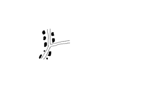
- Buildings are arranged in a line.
Factors:
- Presence of a transport line e.g., road or railway.
- Presence of a river or a spring to provide water for domestic or commercial use.
- Presence of a coastline which has a favourable fishing ground e.g., shore of East African coast.
- Suitable terrain for cultivation of crops such as at the foot of a scarp.
c) Dispersed/Scattered Settlement
- Buildings are scattered.
Factors:
- Plenty of land to build whenever they want.
- Avoidance of harsh climate e.g., arid and semi-arid areas.
- Poor infertile soils.
- Pests and diseases.
- Physical features such as ridges, valleys which separate houses.

d) Radial Pattern
Buildings are arranged like a star.
Common at crossroads where housing units point in all directions.
Enlargement and Reduction of Maps
Steps
- Identify the area requiring to be enlarged.
- Measure its length and width.
- Multiply (E) or divide (R) by the number of times given. The scale also changes e.g., 1:50000 / 2 (enlarged) × 2 (reduced).
- Draw the new frame with new dimensions.
- Insert the grid squares e.g., 2×2 cm, 2/2, etc.
- Draw diagonals on the frame.
- Transfer features exactly where they were.
Drawing a Cross Section/Profile
A line drawn on a piece of paper showing the nature of relief of a particular area.
Steps
- Identify the given points and name them A and B.
- Join points A and B using a pencil.
- Take a piece of paper and fold it into two parts.
- Place the paper’s edge along the line joining A and B.
- Mark all contours and their heights.
- Mark features along A-B e.g., R – river, H – hill, M – mountain.
- Determine the highest and lowest contour height to determine the appropriate vertical scale.
- Draw horizontal axis and mark it A-B.
- Draw vertical axis from A to B.
- Place the edge of folded paper along horizontal axis.
- Use values along vertical axis to plot contour heights. Remember to show features marked along A-B.
- Join plotted points using smooth curve (cross section).
- Include title on top, vertical and horizontal map scale.
Calculation and Interpretation of Vertical Exaggeration and Gradient
Vertical Exaggeration
Number of times that the vertical scale is larger than horizontal scale.
V.E. = Denominator of H.S. / Denominator of V.S. (cross section scale)
e.g., V.S. = 1:20M
H.S. = 1:50000
V.E. = 50000 / 20 × 100 (To convert into cm) = 25
Interpretation
The vertical height has been exaggerated 25 times compared to the horizontal distance.
Intervisibility
Ability of one place to be seen from another.
Steps
- Draw cross section.
- Join points A-B using visibility line.
- If the visibility line is above the cross section, the two points are intervisible. If below, they are not intervisible.
Gradient
Degree of steepness of a slope between two given points.
Steps
- Identify the two points.
- Calculate difference in height between the two points (Vertical Interval) e.g., 500 m.
- Join them with a light line.
- Measure ground distance between the two points (Horizontal Equivalent) e.g., 12 cm.
G = V.I. / H.E.
= 500 × 100 / 12 × 50000 = 50000 / 600000 = 1/12 = 1:12
Interpretation
For every 12 m travelled on the ground, there is a vertical rise of 1 m.


3 Comments