
CHAPTER 2
SPREADSHEETS
This chapter introduces the student to what spreadsheets are, their components, application areas, and practical usage.
Contents
- 2.0 Definition of Spreadsheets
- 2.1 Components of a Spreadsheet
- 2.2 Application Areas of Spreadsheets
- 2.3 Create and Edit a Spreadsheet
- 2.4 Explain Different Cell Data Types
- 2.5 Apply Cell Referencing
- 2.6 Apply Functions and Formulae
- 2.7 Apply Data Management Skills
- 2.8 Apply Charting and Graphing Skills
- 2.9 Print Worksheet and Graph
2.0 Definition of Spreadsheets
A spreadsheet is a grid that organizes data into columns and rows. Spreadsheets make it easy to display information, and people can insert formulas to work with the data. The columns are marked by letters and the rows are marked by numbers. For example, columns A, B, C; beyond letter 26 (i.e., Z), the columns are marked as AA, AB, etc. The intersection of a row and a column is often known as a cell. Each cell has a name known as a cell reference. Each cell is named by the column and the row in which the cell falls under. For example, Cell A3 means that it is on column A and row 3. The cell where the cursor is placed for operations is known as the active cell.


2.1 Components of a Spreadsheet
A spreadsheet is made up of three key components: worksheet, database, and graphs.
2.1.1 Worksheet
A spreadsheet is made up of many worksheets as shown above in the sheet tab. The total sum of all the worksheets makes up a workbook. The figure above is a workbook. Each of these worksheets may hold different sets of information. You can add as many worksheets as you wish in a workbook.
2.1.2 Database
A spreadsheet can hold many records properly ordered in a given format. These records are about particular people or things which make up the records, classified under specified fields. This is a database. Such records are related and could be placed together in one worksheet to mean a file of an entity.
2.1.3 Graphs
A spreadsheet provides a pictorial representation of data in the form of a graph. This is a key feature of a spreadsheet. Whereas words describe analysed data, graphs provide a quick way to visualize the same output.
2.2 Application Areas of a Spreadsheet
Spreadsheets are often used in the following application areas:
- Statistical data analysis
- Accounting
- Data management
- Forecasting (what-if analysis)
- Scientific application
2.2.1 Statistical Analysis
2.2.2 Accounting
2.2.3 Data Management
2.2.4 Forecasting (what-if analysis)
2.2.5 Scientific Application
2.3 Creating a Worksheet/Workbook
2.3.1 Getting Started
For purposes of this syllabus, we shall use Microsoft Office Excel (MS-Excel).
- Go to Start button
- Click Microsoft Office Excel
- The worksheet below will open
2.3.2 Worksheet Layout
The following worksheet loads when you click on MS-Excel.
The parts of this worksheet have been explained above, section 2.0. The menus will be explained as we move along. The Office button, operations buttons such as Exit, Minimize, Maximize, and Restore remain the same as in MS-Word.

2.3.3 Running the Program
Practical Learning: Starting Microsoft Excel To start Microsoft Excel, from the Taskbar, click Start → (All) Programs → Microsoft Office → Microsoft Office Excel.
The Office Button Introduction When Microsoft Excel opens, it displays an interface divided into various sections. The top section displays a long bar also called the title bar. The title bar starts on the left side with the Office Button If you position the mouse on it, a tooltip would appear:
The Options of the Office Button When clicked (with the mouse’s left button), the Office Button displays a menu:
As you can see, the menu of the Office Button allows you to perform the routine Windows operations of a regular application, including creating a new document, opening an existing file, or saving a document, etc. We will see these operations in future lessons. If you right-click the Office Button, you would get a short menu:
We will come back to the options on this menu. The Quick Access Toolbar Introduction On the right side of the Office Button, there is the Quick Access Toolbar Like a normal toolbar, the Quick Access displays some buttons. You can right-click the Quick Access toolbar. A menu would appear:
If you want to hide the Quick Access toolbar, you can right-click it and click Remove Quick Access Toolbar. To know what a button is used for, you can position the mouse on it. A tooltip would appear. Once you identify the button you want, you can click it. Adding a Button to the Quick Access Toolbar By default, the Quick Access toolbar is equipped with three buttons: Save, Undo, and Redo. If you want to add more buttons or options, you can right-click the Quick Access toolbar and click Customize Quick Access Toolbar… This would display the Excel Options dialog box:
To add a button to the Quick Access toolbar, on the left list of Add, click an option and click Add. After making the selections, click OK. To remove a button from the Quick Access toolbar, right-click it on the Quick Access toolbar and click Remove From Quick Access Toolbar. The Quick Access Button On the right side of the Quick Access toolbar, there is the Customize button with a down-pointing arrow. If you click or right-click this button, a menu would appear:
The role of this button is to manage some aspects of the top section of Microsoft Excel, such as deciding what buttons to display on the Quick Access toolbar. For example, instead of using the Customize Quick Access Toolbar menu item as we saw previously, you can click an option from that menu and its corresponding button would be added to the Quick Access toolbar. If the options on the menu are not enough, you can click either Customize Quick Access Toolbar or More Commands… This would open the Excel Options dialog box. The main or middle area of the top section displays the name of the application: Microsoft Excel. You can right-click the title bar to display a menu that is managed by the operating system. On the right side of the title bar, there are three system buttons that allow you to minimize, maximize, restore, or close Microsoft Excel. Under the title bar, there is another bar with a Help button on the right side. The Ribbon Introduction Under the title bar, Microsoft Excel displays a long bar called the Ribbon:
Minimizing the Ribbon By default, the Ribbon displays completely in the top section of Microsoft Excel under the title bar. One option is to show it the way the main menu appeared in previous versions of Microsoft Excel. To do this:
This would display the Ribbon like a main menu:
To show the whole Ribbon again:
Changing the Location of the Ribbon By default, the Quick Access toolbar displays on the title bar and the Ribbon displays under it. If you want, you can switch their locations. To do that, right-click the Office Button, the Quick Access toolbar, or the Ribbon, and click Show Quick Access Toolbar Below the Ribbon:
To put them back to the default locations, right-click the Office Button, the Quick Access toolbar, or the Ribbon, and click Show Quick Access Toolbar Above the Ribbon. The Tabs of the Ribbon The ribbon is a type of property sheet made of various property pages. Each page is represented with a tab. To access a tab:
To identify each tab of the Ribbon, we will refer to them by their names. The Sections of a Tab Each tab of the ribbon is divided into various sections, each delimited by visible borders of vertical lines on the left and right. Each section displays a title on its bottom side. In our lessons, we will refer to each section by that title. For example, if the title displays Font, we will call that section “The Font Section”. Some sections of the Ribbon display a button The Buttons of the Ribbon Since there are various buttons and sometimes they are unpredictable, to know what a particular button is used for, you can position your mouse on it. A small box would appear to let you know what that particular button is used for; that small box is called a tooltip:
You can also use context-sensitive help in some cases to get information about an item. You can add a button from a section of the Ribbon to the Quick Access toolbar. To do that, right-click the button on the Ribbon and click Add to Quick Access Toolbar:
Remember that, to remove a button from the Quick Access toolbar, right-click it on the Quick Access toolbar and click Remove From Quick Access Toolbar. The More Buttons of the Ribbon In some sections of the Ribbon, on the lower-right section, there is a button:
That button is used to display an intermediary dialog box for some action. We will see various examples as we move on. The Size of the Ribbon When Microsoft Excel is occupying a big area or the whole area of the monitor, most buttons of the Ribbon appear with text. Sometimes you may need to use only part of the screen. That is, you may need to narrow the Microsoft Excel interface. If you do, some of the buttons may display part of their appearance and some would display only an icon. Consider the difference in the following three screenshots:
In this case, when you need to access an object, you can still click it or click its arrow. If the item is supposed to have many objects, a new window may appear and display those objects: From this:
To this:
The Work Area The Name Box Under the Ribbon, there is a white box displaying a name like A1 (it may not display A1…), that small box is called the Name Box:
The Insert Function Button On the right side of the Name Box, there is a gray box with an fx button. That fx button is called the Insert Function button. The Formula Bar On the right side of the Insert Function button is a long empty white box or section called the Formula Bar:
You can hide or show the Formula Bar anytime. To do this, on the Ribbon, click View. In the Show/Hide section:
The Column Headers Under the Name Box and the Formula Bar, you see the column headers. The columns are labeled A, B, C, etc:
There are 255 columns. The Row Headers On the left side of the main window, there are small boxes called row headers. Each row header is labeled with a number, starting at 1 on top, then 2, and so on:
The Cells The main area of Microsoft Excel is made of cells. A cell is the intersection of a column and a row:
A cell is identified by its name and every cell has a name. By default, Microsoft Excel appends the name of a row to the name of a column to identify a cell. Therefore, the top-left cell is named A1. You can check the name of the cell in the Name Box. Practical Learning: Using Cells
The Scroll Bars On the right side of the cells area, there is a vertical scroll bar that allows you to scroll up and down in case your document cannot display everything at a time:
In the lower right section of the main window, there is a horizontal scroll bar that allows you to scroll left and right if your worksheet has more items than can be displayed all at once:
Sometimes the horizontal scroll bar will appear too long or too narrow for you. If you want, you can narrow or enlarge it. To do this, click and drag the button on the left side of the horizontal scroll bar:
The Sheet Tabs On the left side of the horizontal scrollbar, there are the worksheet tabs:
By default, Microsoft Excel provides three worksheets to start with. You can work with any of them and switch to another at any time by clicking its tab. The Navigation Buttons On the left side of the worksheet tabs, there are four navigation buttons:
If you happen to use a lot of worksheets or the worksheet names are using too much space, which would result in some worksheets being hidden under the horizontal scroll bar, you can use the navigation buttons to move from one worksheet to another. The Status Bar Under the navigation buttons and the worksheet tabs, the Status Bar provides a lot of information about the job that is going on. |

 .
.


 .
.


 . If you see such a button, you can click it. This would open a dialog box or a window.


Microsoft Excel File Operations
Saving a File
A Microsoft Excel file gets saved like any traditional Windows file.
To save a file:
- You can press Ctrl + S
- On the Quick Access Toolbar, you can click the Save button

- You can click the Office Button and click Save


Two issues are important. Whenever you decide to save a file for the first time, you need to provide a file name and a location. The file name helps the computer identify that particular file and register it.
A file name can consist of up to 255 characters. You can include spaces and dashes in a name. Although there are many characters you can use in a name (such as exclamation points, etc.), try to avoid fancy names. Give your file a name that is easily recognizable and a little explicit. For example, such names as Time Sheets, Employee’s Time Sheets, GlobalEX First Invoice are explicit enough. Like any file of the Microsoft Windows operating systems, a Microsoft Excel file has an extension, which is .xls, but you don’t have to type it in the name.
The second important piece of information you should pay attention to when saving your file is the location. The location is the drive and/or the folder where the file will be saved. By default, Microsoft Excel saves its files in the My Documents folder. You can change that in the Save As dialog box. Just click the arrow of the Save In combo box and select the folder you want.
Microsoft Excel allows you to save its files in a type of your choice.
To save a file in another format:
- Press F12 or Shift + F12
- You can click the Office Button and position the mouse on Save As and select the desired option:
- On the Quick Access Toolbar, you can click the Save button . Then, in the Save As dialog box, click the arrow of the Save As Type combo box and select a format of your choice

 . Then, in the Save As dialog box, click the arrow of the Save As Type combo box and select a format of your choice
There are other things you can do in the Save As dialog box:

Practical Learning: Saving a File
- To save the current document, on the Quick Access Toolbar, click the Save button
- Type Fundamentals
- Click the Save button

Saving under a Different Name and New Folder
You can save a file under a different name or in another location. This gives you the ability to work on a copy of the file while the original is intact.
There are two primary techniques you can use to get a file in two names or the same file in two locations. When the file is not being used by any application, in Windows Explorer (or in My Computer, or in My Network Places), locate the file, right-click it and choose Copy.
To save the file in a different name, right-click in the same folder and choose Paste. The new file will be named Copy Of… You can keep that name or rename the new file with a different name (recommended).
To save the file in a different location, right-click in the appropriate folder and click Paste; in this case, the file will keep its name.
In Microsoft Excel, you can use the Save As dialog box to save a file in a different name or save the file with the same name (or a different name) in another folder. The Save As dialog box also allows you to create a new folder while you are saving your file (you can even use this technique to create a folder from the application even if you are not saving it; all you have to do is create the folder, click OK to register the folder, and click Cancel on the Save As dialog box).
Practical Learning: Save a File With Different Settings
- To save this file using a different name, click the Office Button, position the mouse on Save As, and click Excel 97-2003 Workbook
- Change the name of the file to Employment Application
- On the toolbar of the Save As dialog box, click the Create New Folder button (if you have a hard time finding it, press Alt + 5)
- Type My Workbooks and press Enter. The My Files folder should now display in the Save In combo box. If you clicked Cancel or pressed Esc now to dismiss the Save As dialog box, the computer would still keep the folder
- After making sure that the My Files folder displays in the Save In combo box, click the Save button
Opening a File
The files you use could be created by you or someone else. They could be residing on your computer, on another medium, or on a network. Once one of them is accessible, you can open it in your application.
You can open a document either by double-clicking its icon in Windows Explorer, in My Computer, from the Find Files or Folders window, in My Network Places, or by locating it in the Open dialog box.
To access the Open dialog box, on the main menu, click File → Open…
You can also click the Open button on the Standard toolbar.
A shortcut to call the Open dialog box is Ctrl + O.
2.4 Cell Data Types
The data that you enter in a cell can take any of the following four types:
- Labels – these are data which are in text form. For example, titles on top of the columns or at the start of each row.
- Values – these are the result from a calculation. They are often in the form of numbers, currencies, dates, and so on.
- Formulae – these are data that use operators such as +, -, /, *, brackets.
- Functions – these are the cell data types which contain the formulae which the spreadsheet has memorized and is available in the library. A function usually contains an equal sign (=), function name such as SUM, AVERAGE, MAXIMUM, and so on, and values to be used with the function. An example of a function in a cell would be: =SUM(A2:A4).
2.5 Cell Referencing
2.5.1 Cell Addressing
A cell must have a cell address, the name of the cell. The cells are addressed using column letter and row number. For example, cell A3 means a cell positioned on column A and row 3. Microsoft Excel, just like any other spreadsheet, works with cell references instead of values. This is because the references provide an easy way to amend contents of a cell instead of the values.
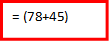
Example of use of a cell reference:
The first uses cell references to add the two numbers. When this happens, you can easily change the contents of any of the two cells, and immediately the answer will change to correspond with the change you have made. In the second formula, even if you change the content of the formula, the answer will not change at all.


2.5.2 Absolute Referencing
A cell whose contents need to remain constant throughout the calculation period is referred to as an absolute reference. It is usually denoted by a dollar sign, thus, $B$2. This can be done simply by highlighting the cell reference and then pressing F4 on the keyboard to add the dollar signs.


