THEORY OF DEMAND
- Demand refers to quantity of the goods and services consumers are able and willing to purchase at the prevailing price in a given period of time.
- According to Bober: “By demand we mean the various quantities of a given commodity or service which consumers would buy in one market in a given period of time at various prices or at various incomes, or at various prices related goods.”
- From the point of view of the seller, the demand price is the average revenue (revenue per unit) or income he expects to earn from the sale of unit of a commodity. Thus, demand price is identical with average revenue (AR). That is why the demand curve is also drawn as AR curve.
The law of demand states that “The higher the price the lower the demand, the lower the price the higher the demand, other factors remaining constant.”
Assumptions of the law of demand
The law of demand operates when all factors affecting demand apart from the price of the commodity are kept constant, therefore the following are the assumptions of the law of demand:
- No change in the level of distribution of income
- The consumer’s level of income remains the same
- Population size remains unchanged
- The prices of other related goods remains the same
- There is no change in taste and preferences
- The level of advertisement remains the same
- The level of income tax remains unchanged
The Demand Schedule
This is the table that shows different price levels and the corresponding quantities demanded of the commodity.
| Price of milk per ltr in Tshs. | 100 | 200 | 300 | 400 |
| Quantity demanded of milk in ltrs | 8 | 6 | 4 | 1 |
Types of Demand Schedule
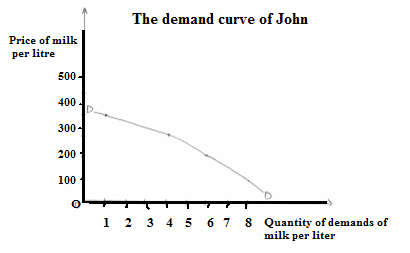
- Individual demand schedule – This is the type of table which shows different quantities demanded of the commodity by an individual.
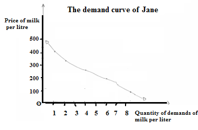
- Market demand schedule – This is the table which shows different total quantities demanded of the commodity at different prices in the whole market.
NOTE. In order to get a market demand schedule we add up individual demand schedules.
| Price of milk per ltr | Qty demanded milk by John in ltr | Qty demanded of milk by Jane ltrs | Market demand |
| 100 | 8 | 6 | 14 |
| 200 | 6 | 4 | 10 |
| 300 | 4 | 2 | 6 |
| 400 | 1 | 1 | 2 |
Assuming there are two buyers in the market for milk, John and Jane, the market demand schedule will be derived as above.
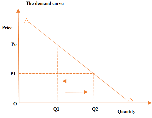
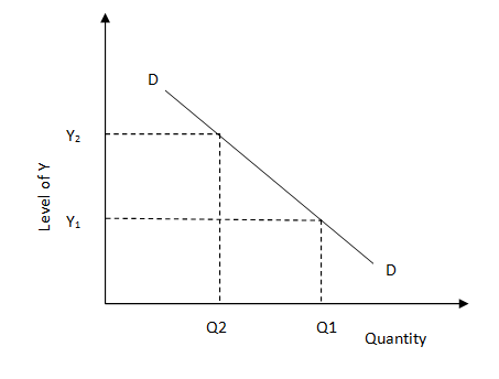
The Demand Curve
This is a graphical presentation of the demand schedule showing the relationship between price of the commodity and its demand.
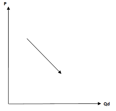
A demand curve has a negative slope and slopes downwards from left to right showing that as the price decreases the quantity demanded increases, other factors remaining constant.
The demand curve
The demand curve of Jane
The market demand curve
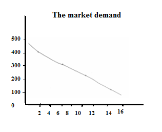
FACTORS AFFECTING DEMAND
Demand of a good or service will be high or low depending on the following factors:
- The price of the commodity.
When the price of the commodity is high the demand will be low, and when the price is low demand will be high, other things being constant.
- Population size
The demand in an area with high population will be high while the demand in an area with low population will be low.
- Consumer’s level of income
When the consumer’s level of income is high, the demand will be high as the consumer’s ability will be high. However, when the consumer’s level of income is low, the demand will also be low as the consumer’s ability will be low.
- Level of advertisement
The commodity which is extensively advertised will be highly demanded, while the commodity which is not advertised will have low demand.
- Tastes and Preference
If the commodity is favored by people’s taste and preference, the demand will be high while the commodity which is not favored by people’s tastes and preference will have low demand.
E.g., the demand of Hijab in Saudi Arabia is higher compared to the demand in the USA.
- The level of Taxation
When the income tax charged is high, demand will be low and when the income tax is low, demand will be high, as the disposable personal income will be high.
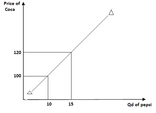
- The price of the substitute goods
If the price of the substitute increases, demand of the good will decrease and when the price of the substitute decreases, the demand of the good will increase.
Substitutes are goods for which one can be used instead of the other, e.g., Pepsi and Coca-Cola.
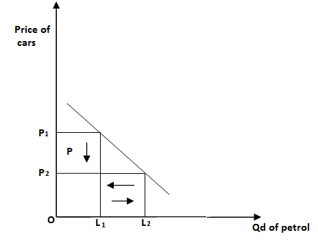
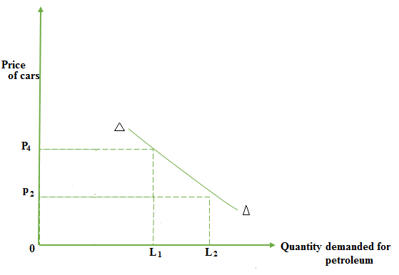
- Price of the complement
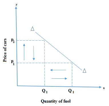
Complement goods are jointly demanded. These are goods where the demand of one results in demand for the other, e.g., Car & petrol.
If the price of the complement is high, the demand of the good in question will be low and when the price of the complement is low, the demand of the good in question will be high. (e.g., When the price of a car is high, demand for petrol will be low and when the price of the car is low, demand for petrol will be high.)
- Season
The demand of some goods is seasonal in nature. When the prevailing season favors certain goods, its demand will be high and when the prevailing season does not favor a certain good, its demand will be low.
E.g., The demand of woolen jackets in winter will be high compared to the demand of woolen jackets in summer which will be low.
The downward sloping demand curve
The demand curve slopes downwards from left to right (negative slope). This indicates that more is demanded as the price falls and less is demanded when the price increases. Such negative slope is due to the following factors:
- Income effect
As the price falls, real income increases and therefore consumers can now buy more units of a commodity with the same income. On the other hand, when the price increases, real income decreases and therefore consumers can now buy fewer units with the same income.
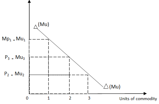
- The law of diminishing marginal utility
The law of diminishing marginal utility states that “as more and more units of the commodity are consumed, the additional satisfaction goes on declining.” Therefore, more and more units of the commodity will be purchased only if the price is falling.
- Substitution effect
When the price of the commodity is low, it becomes cheaper in comparison to other competing commodities and the consumers start to substitute this commodity in place of other commodities; therefore demand for the commodity increases with the fall in price.
- New customers
When the price of the commodity falls, new customers join buying that commodity, those who could not afford before, hence increase in demand. On the other hand, when the price rises, some old customers may stop purchasing the commodity and hence fall in demand.
Uses of the commodity
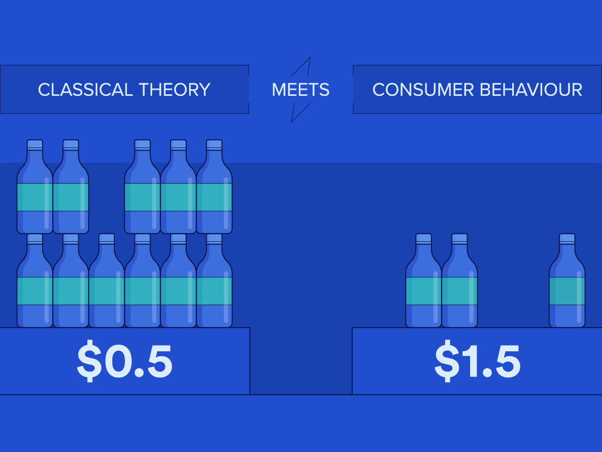
- A commodity tends to have more uses or less urgent uses when it becomes cheaper. For example, if water is dear, we shall use it for drinking only, but when it becomes cheaper, we shall use it for washing and other less urgent uses.
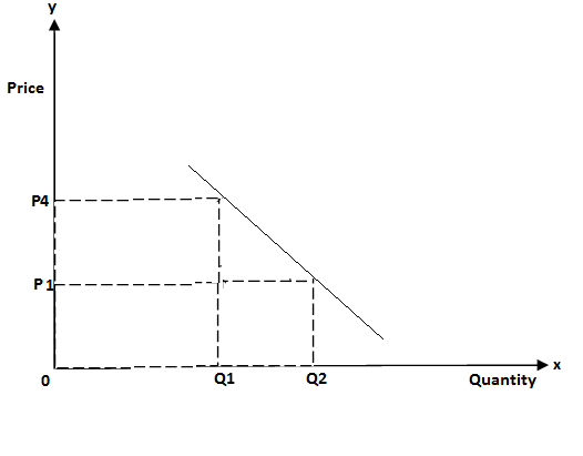
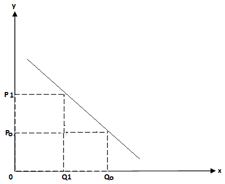
Change in quantity demanded and change in demand
Change in quantity demanded
- This means increase or decrease in quantity demanded due to change in the price of the commodity, other factors remaining constant.
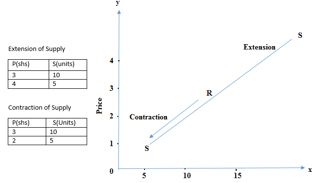
- It is illustrated through the movement along the same demand curve. Through extension it is increase in Qd and contraction is the decrease in Qd.
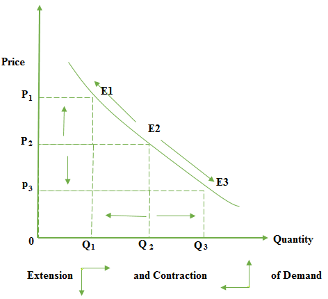
Let us assume the economy in equilibrium at point “E2” that is at price “OP2” and quantity demand is “OQ2”.
Case I (contraction of demand)
Let us assume that the price increases from “OP2” to “OP1” and the quantity demand reduces from “OQ2” to “OQ1”. This behavior is referred to as “Contraction of demand”.
- Case II (Extension of demand)
In this case the price decreases from “OP2” to “OP3”. Due to this, the quantity demand increases from “OQ2” to “OQ3”. This is nothing but the extension of demand.
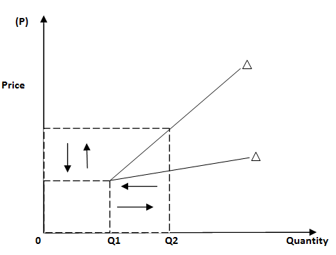
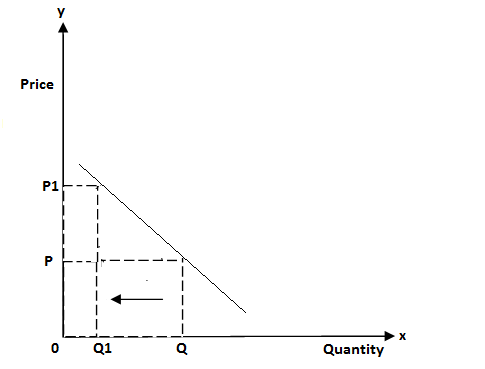
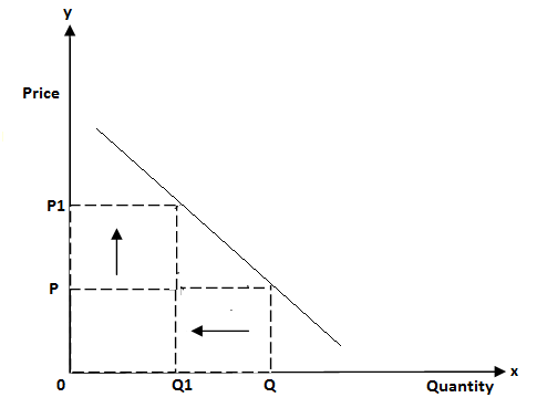
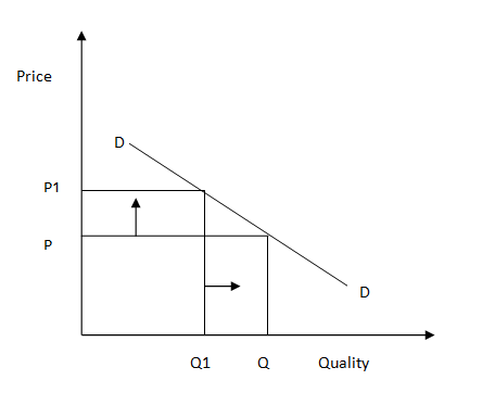
Change in demand
Is the increase or decrease in demand due to change in all the factors affecting demand apart from the price.
It is illustrated through the shift of the demand curve either to the right (increase in demand) or to the left (decrease in demand).
In the diagram, “dd” is original demand curve. “dd” is decrease in demand curve. “” is increase in demand curve, “OP” original price, “OQ” original quantity.
“OP” Original Price “OQ1” Increase in demand.
“OP” Original Price “OQ2” Increase in demand.
REASONS FOR CHANGE IN DEMAND
- Change in the consumer’s level of income
When the consumer’s level of income increases, demand will also increase because of the increase in purchasing ability and when the level of income decreases, demand will decrease due to decrease in purchasing ability.
- Change in population size
When the population size increases, demand will also increase because of more consumers and when the population decreases, demand will also decrease due to fewer consumers.
- Change in the level of direct taxes
When the level of direct tax increases, demand will decrease due to the decrease of disposable personal income and when the level of direct taxes decreases, demand will increase due to the increase of disposable personal income.
- Expectation or Anticipations
Expectations also bring about a change in demand. If prices are expected to rise in future, the demand for goods will increase now in the present. Similarly, expectation of rising incomes will restrain current purchases and postpone purchases to a future favorable situation.
- Change in tastes, preferences and fashion
When the tastes, preferences & fashion change in favor of certain goods, demand will increase and when the taste, preferences & fashion change against a certain good, its demand will decrease.
- Change in price of the substitute
If the price of the substitute increases, the demand of a good in question will increase and if the price of the substitute decreases, the demand of a good in question will decrease.
- Change in the price of the complement
If the price of the complement increases, the demand of the good in question will decrease. However, if the price of the complement decreases, the demand of the good in question will increase.
8. Exceptions of the law of Demand
There are some situations where the law of demand does not operate. This gives rise to abnormal demand curve (regressive).
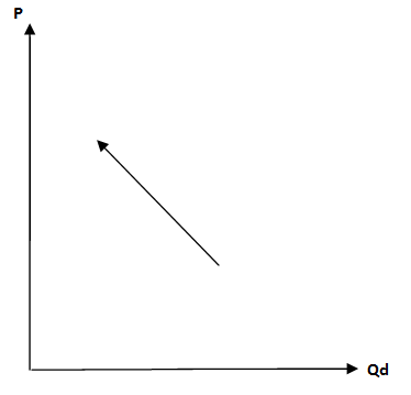
Aggressive demand curve has a positive slope indicating that as the price increases quantity demand also increases and vice versa. A situation which is against the law of demand.
The exceptions of the law of demand are the following:
9. Veblen goods or Article of ostentation
These are the luxurious goods which are demanded to emphasize economic status, for example expensive cars, expensive mobile phones etc. For such goods, as the price increases, quantity demanded also increases.
Giffen goods (inferior goods)
This can also be called inferior goods, examples of such include maize flour. For such goods, when the price increases, more is bought of them, but as the price falls, less is demanded of them. For a low income earner, when the price of beans increases, he will buy more of them by reducing his expenditure on meat.
- Fear of the future rise in price
When the consumers expect the price of the commodity to increase now and then because of factors such as expected shortage, they will tend to buy more of the commodity as the price increases.
- Necessities
These are goods that are necessities of life, e.g., medicines, food, salt etc.
For such goods, a minimum quantity has been purchased by the consumer irrespective of their price because of such a situation, the law of demand is operative to a certain extent.
- Ignorance of the consumer
These are situations where consumers buy goods at a higher price because they are ignorant of lower prices for the same goods in other markets.
Interrelated Demand
Under inter-related demand, we examine the relationship between goods that are related in one way or another by looking at how change of one will affect demand of the other.
Types of Inter-related Demand
- Joint Demand (complementary demand)
This is the demand for two or more commodities which are jointly needed to satisfy a particular need.
Example: Car and petrol. Increase in demand of one will result in increase in demand for another and decrease in demand of one will result in decrease in demand for another. Increase in the price of one will result in decrease in demand for another.
- Competitive Demand
This refers to the demand for goods which are substitutes to one another. For example tea and coffee, Pepsi and Coca-Cola. Increase in demand for one will result in decrease in demand for another and vice versa. Increase in price for one will result in increase in demand for another and vice versa.
- Composite Demand
This refers to demand for a commodity which can be used for several purposes e.g., demand for electricity, demand for steel.
- Derived Demand
This refers to demand for a commodity which is used in the production of another commodity. E.g., demand for factors of production is derived demand because it is upon demand for goods that produces demand for factors of production in order to produce other goods.
Elasticity of Demand
Definition
Elasticity of Demand is the responsiveness of demand to change in price.
Types of Elasticity
There are basically three types of elasticity:
- Price Elasticity of Demand
- Income Elasticity of Demand
- Cross Elasticity of Demand
A. Price Elasticity of Demand
Is the responsiveness of demand to change in price level. It measures responsiveness of potential buyer to change in price.
Price elasticity can be measured by the help of the following formula:
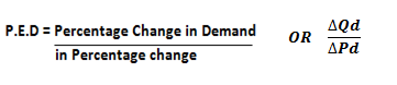
Price elasticity is always negative.
Interpretation of Price Elasticity of Demand
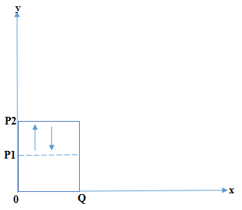
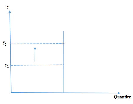
- Perfectly inelastic (P.E.D = 0)
This means that change in price has no effect on quantity demanded.
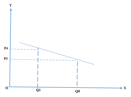
- Inelastic (P.E.D < 1)
This means that a big change in price brings about a small change in demand.
- Unitary (PED = 1)
This means that a change in price results in an equal change in demand.
- Elastic (PED > 1)
This means that a small change in price results in a big change in demand.
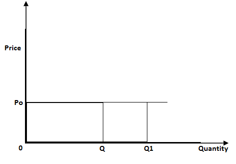
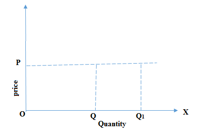
- Perfect Elastic (PED = ∞)
This means that price is not changing (fixed) but quantity demanded is changing.
FACTORS WHICH INFLUENCE PRICE ELASTICITY OF DEMAND (PED)
PED can be elastic or inelastic depending on the following factors:
Degree of availability of close substitutes
If a commodity has many close substitutes, its price elasticity of demand will be elastic as consumers can easily move over to other alternatives. However, if commodities have few substitutes, its demand will be inelastic.
- Proportion of income spent on a good
If the commodity takes a large percentage of someone’s income, its demand will be price elastic as increase in the price can easily be felt. However, if a commodity takes a small percentage of someone’s income e.g., matchbox, its demand will be price inelastic.
The level of Income
With a high level of income, demand will be price inelastic since increase in the price can easily be absorbed. On the other hand, with a lower level of income, the demand will be low hence price is inelastic.
Time period
In the short run, demand would be price inelastic as the consumer will not be able to gain enough market information e.g., the prices of other competing goods. However, in the long run, demand would be price elastic as the consumer would have gained enough market information e.g., the price of substitutes.
The degree of necessity
If the commodity is a necessity, its demand would be price inelastic as a person cannot easily do without them. On the other hand, luxurious goods have elastic demand.
Habit
For goods with addiction in their consumption e.g., cigarettes, alcohol, their demand is price inelastic; however, those goods with no addiction have price elastic demand.
Durability of a commodity
Durable goods such as furniture have inelastic demand, since they can stand for a long period of time after being bought. On the other hand, non-durable goods have elastic demand.
Importance or Practical application of P.E.D
- To the primary decision
P.E.D is important to business in pricing decision making in order to maximize total revenue (TR). Therefore, it is on the basis of the price elasticity of demand of the commodity that a seller will decide whether to increase or reduce the price (P) in order to maximize total revenue as below:
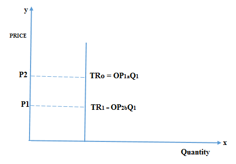
When PED is perfectly inelastic, he should increase the price to earn revenue since demand will remain exactly the same.
When P.E.D is inelastic, the business should decrease the price in order to earn total revenue because at such high price, demand will remain almost the same.
When price elasticity of demand is unitary, the business should leave the price the same since increase or decrease in the price will lead to the total revenue being the same.
When P.E.D is elastic, a businessman should reduce the price in order to earn more revenue because decrease in price sparks off a big increase in demand.
2. To a Monopoly
When carrying out price discrimination, the monopolist considers the price elasticity of demand in the market in order to decide in which market to charge a high price and in which to charge low price. In that market where price is elastic, he should charge a low price and in that market where price is inelastic, he should charge a high price.
3. Wage Determination
Elasticity of demand for labor is important in wage determination in such a way that when demand for labor in a firm is inelastic, trade unions and laborers can easily succeed in bargaining for high wages than when the elasticity of demand of labor is elastic.
4. Government in Taxation
The government uses the concept of price elasticity of demand in determining which commodity to levy high tax and which to levy low taxes in order to collect more revenue. Those goods whose demand is price inelastic e.g., cigarettes, alcohol etc., the government will levy high taxes. However, for the goods whose demand is price elastic, the government will levy low taxes.
5. Determination of incidence of a tax
Determination of the incidence of a tax between producer and the buyer is on the basis of the price elasticity of demand of the commodity as below.
Demand for the commodity is price inelastic, the bigger the burden is borne by the buyer and the smaller one by the producer.
If elasticity of demand is unitary, the burden is shared equally between the producer and the buyer.
If demand for the commodity is price elastic, the smaller burden is shared equally between the producer and the buyer.
If demand for the commodity is price inelastic, the smaller burden is borne by the buyer and the bigger burden is borne by the producer.
6. Under International Trade (devaluation)
Devaluation is the deliberate action by the government to lower the value of its currency in relation to foreign currency. It aims at increasing export and reducing import; however, this is only possible if the price elasticity of demand of both exports and imports is elastic.
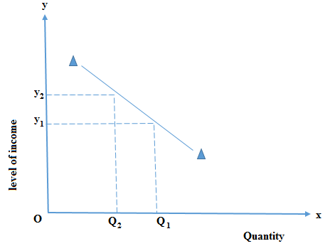
A. Income Elasticity of Demand
This is the measure of degree of responsiveness of demand due to change in the consumer’s level of income.
I.E.D = (proportionate change in demand) / (proportionate change in income)
OR
ΔY = Changing income
Yo = Income before change
Q = Quantity
Interpretation of Income Elasticity
- YED = -ve
This means that a commodity is an inferior good whereby as the income increases quantity decreases.
- Y.E.D = +ve
This means that a commodity is a normal good; therefore, as the level of income increases, demand increases (Articles of Ostentation).
- YED = 0
This means that the commodity in consideration is a necessity e.g., medicine etc., therefore as the level of income increases, demand remains constant.
- YED < 1 (inelastic income elasticity)
This means that a big change in the level of income results in a small change in demand. This is applicable under necessities.
- YED > 1 (elastic income elasticity)
This means that a small change in the level of income results in a big change in demand. This is applicable for inferior goods.
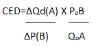
3. Cross Elasticity of Demand (CED)
This is a measure of degree of responsiveness of demand of a good due to change in price of any substitute commodity.
C.E.D = Percentage change in demand for good “A” / Percentage change in price of another product “B”
Interpretation of Cross Elasticity of Demand
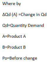
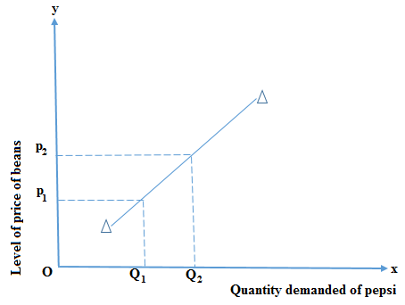
- CED = +ve
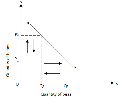
This means the commodity in consideration is a close substitute e.g., beans and peas; therefore, when the price of one increases, demand of the other increases and vice versa.
- CED = -ve
This means that two commodities in consideration are complements (jointly demanded) e.g., car and petrol. For such goods, when the price of one increases, demand for the other decreases and vice versa.
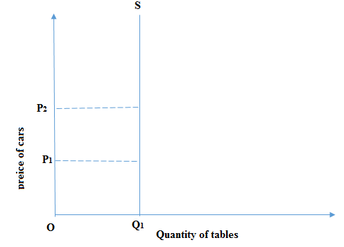
- CED = 0
This means that the two commodities in consideration are not related at all; therefore, a change in the price of one does not bring about any change in demand of the other e.g., car and table.
Arc and Point Elasticity
Arc Elasticity
According to Baum, “Arc Elasticity is a measure of the average responsiveness to price change exhibited by a demand curve over some finite stretch of the curve.”
Or
Arc elasticity is an estimate of the elasticity along average of demand curve. It can be calculated for both linear and non-linear demand curves using the following formula.
Arc.e.d = – ΔQ × (P1 + P2)/2 ÷ ΔP × (Q1 + Q2)/2
Or
Arc eD = difference in Q × difference in P ÷ sum of Q × sum of P
Therefore Arc e.D = (Q1 – Q2) ÷ (P1 – P2) × (Q1 + Q2) ÷ (P1 + P2)
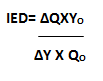
Point Elasticity
Point Elasticity of demand is measured by the slope of tangent to the demand curve at that point.
Price elasticity with complete accuracy at a point on the demand curve.
The formula for calculating point elasticity of demand is as follows:
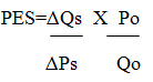
Point ed = -Δq/q ÷ Δp/p = Δq × P0 ÷ Δp × Q0
Factors of Elasticity of Demand
There are several factors which determine the elasticity of demand.
These are the following:
- For necessaries of life demand is less elastic.
As regards the necessaries of life, demand is less elastic because these commodities are purchased at whatever price they may be. Change in price does not matter so far as demand for such commodities is concerned. Wheat and cloth are examples of such things.
- Demand for luxuries is more elastic.
The demand for luxuries is more elastic in the sense that a little change in price level brings a greater change in demand. Television and video sets are examples of such things.
- For substitute demand is more elastic.
The commodities which have their substitutes, their demand is more elastic. For example, when price of tea rises, demand for tea will decrease to great extent because more coffee will be demanded.
- Demand for goods having several uses is more elastic.
The commodities which have various uses have more elastic demand. Coal is such a case; when it is cheap, the use for less urgent needs will extend and when its price rises, it will be put only to more urgent uses and its demand will decrease to a great extent.
- Demand for goods the use of which can be postponed.
Demand for goods, the use of which can be postponed is more elastic. For example, when building material is very costly, the building activities are very much reduced and vice versa.
- Price level
Elasticity also depends upon the price. If the price is either too high or too low, the demand will be less elastic. For example, in the case of cars and salt.
THEORY OF SUPPLY
Supply means the quantity of goods and services a producer is willing and able to offer for sale in the market at the prevailing price per period of time.
The law of supply states that, “The higher the price the higher the supply and the lower the price, the lower the supply, other factors remaining constant.”
Assumptions of the law of supply
The law of supply operates when all factors affecting supply are kept constant apart from the price; therefore, the following are its assumptions.
- The level of technology is constant
- The climatic season remains the same
- The number of producers remains the same
- The government policy remains unchanged
- The price factor of inputs remains fixed
- The level of demand remains the same
- The prices of other related goods remains the same
Supply schedule – Is a table that shows various quantities of goods and services offered for sale at their corresponding prices.
An individual supply – Is a table that shows various quantities of goods and services a single producer is willing and able to offer for sale in the market at different prices per period of time.
Market supply schedule – Is a table that shows different total quantities that producers are willing and able to offer for sale in the market at different prices per period of time.
Note: In order to get a market supply schedule we add up individual supply schedules.
Supply curve – Is a geometrical representation of various quantities offered for sale by producers of a commodity and their corresponding prices.
Note: The supply curve can be an individual or market supply curve; therefore, in order to get a market supply curve we add up individual supply curves.
Factors Affecting Supply
- Price of the commodity
The higher the price of the commodity, the higher the supply; the lower the price of the commodity, the lower the supply, other factors remaining constant.
- Number of producers
If there is a big number of producers of a particular commodity, supply will be high and when there is less number of producers of a particular commodity, supply will be low.
- Production technique (level of production)
With the use of improved and better technology, supply will be high. However, the use of inferior and low level of technology, supply will be low.
- Government policy
Provision of subsidies to producers results in more supply as it lowers the cost of production; on the other hand, imposition of taxes discourages producers and hence low supply.
- Gestation Period (production period)
The shorter the gestation period, the higher the supply and the longer the gestation period, the lower the supply.
- Time
In the short run, supply will be less since some factor inputs will be fixed. However, in the long run, supply will be high as the firm will be able to vary all its factor inputs.
- Price of the substitutes
When the price of the substitute is high, supply of a good in question will be low because of low level of profitability; however, when the price of the substitute is low, supply of a good in question will be high.
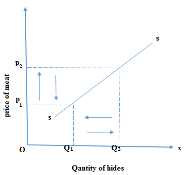
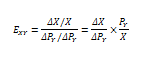
- Price of the complement (Jointly Supplied goods)
When the price of the complement is high, supply of a good in question will be high and the opposite is true. E.g., when the price of meat is high, supply of hides will also be high and vice versa.
Change in Quantity supplied and change in supply
- This means increase and decrease in quantity supplied due to change in the price of the commodity other factors remaining constant.
When the price increases, quantity supplied increases and with the price decrease, quantity supplied decreases.
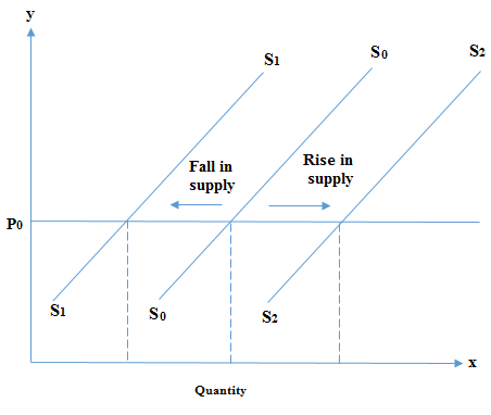
- Also referred to as the shift of the supply curve. This means rise or fall in supply due to all factors affecting supply apart from the price. When the supply curve shifts to the right it means a rise in supply and when it shifts to the left it means decrease/fall in supply.
FACTORS OF CHANGE IN SUPPLY
- Cost of Production
When cost of production of any commodity rises, supply falls and vice versa.
- Climate situation
If climatic situation remains favorable, agricultural production will increase and as a result of this supply will rise and vice versa.
- Improvement in the method of production
When new and less expensive methods of production are invented, supply will increase/rise and vice versa.
- Development of means of transport and communication
If means of transport and communication are adequate and developed, it will be possible to move commodities from one place to another place. In this case supply will rise and vice versa.
- Peace and security
With peace and security, supply rises because production is encouraged and vice versa.
- Policy of the Government
When restrictions are levied by the government on the movement of goods, supply will fall and when such restrictions are removed supply will rise.
- Rates of Taxes
When taxes are levied at a higher rate, supply falls and vice versa.
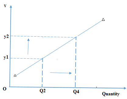
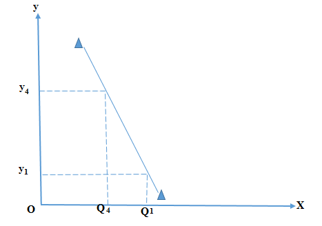
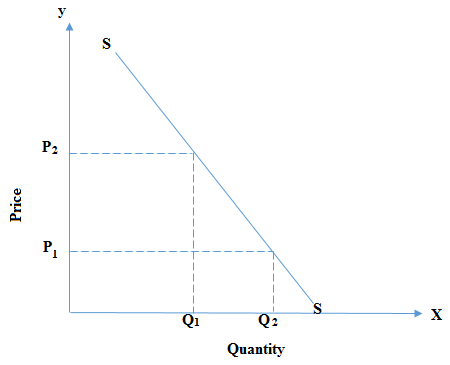
Abnormal Supply curve
Is that supply curve which disobeys the law of supply. It has a negative slope. It implies that the higher the price of the commodity, the lower the quantity supplied of it and vice versa.
The cases of abnormal supply curve are not common. In very rare cases only a supply curve will be of the abnormal shape. There is one good example of abnormal supply curve i.e., the bending supply curve of labor. This shows that beyond a specific wage level, any rise in wages will result in decrease in working hours. The shape of the supply curve of labor is as under.
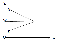
When wages rise beyond OW then working hours decrease.
Inter-related supply
- Joint Supply
Some goods are produced together. The supply of those goods which have common process of production is known as joint supply. The supply of such goods is increased or decreased simultaneously.
E.g. a) Wood and Mutton are produced jointly.
b) From crude oil, different types of petrol production are obtained such as diesel, engine oil, super etc.
- Composite Supply
The goods which are substitutes of one another, their total quantity is called composite supply.
E.g. a) Supply of Mutton, beef and chicken.
b) Supply of Tea and Coffee.
c) Supply of cold drinks like Coca-Cola and Pepsi.
- Competitive Supply
There are some alternative uses of land, labor and capital. If these factors are used for the production of one commodity then the supply of other commodities is affected.
E.g. a) If more land is used to produce wheat then production of maize will decrease. The supply of these goods is competitive supply.
ELASTICITY OF SUPPLY
Elasticity of Supply – Is the measure of the ease with which an industry can be expanded and of the behaviour of the marginal costs.
A. Price Elasticity of Supply
Price elasticity of supply is the measure of degree of responsiveness of supply due to change in price of commodity.
P.E.S = (proportional change in amount supplied) / (proportional change in price)
Interpretation of PES
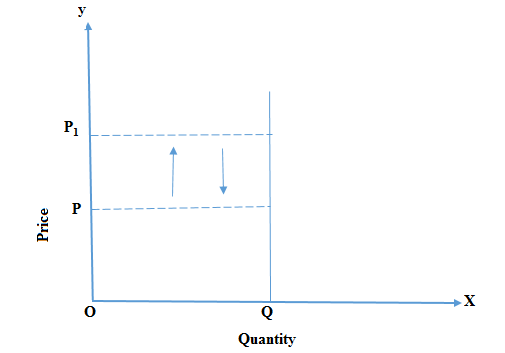
- PES = 0 (perfectly inelastic)
This means there is no change in quantity supplied due to change in price.
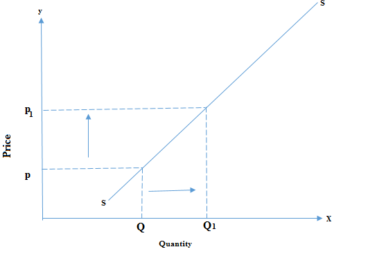
- PES < 1 (inelastic)
This means that the change in price is greater than the change in quantity supplied.
- PES = 1 (unitary)
This means the amount of change in price is equal to the amount of change in quantity supplied.
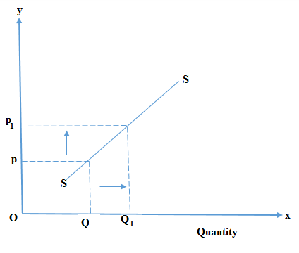
- PES > 1 (elastic)
This means that change in quantity supplied is more than change in price.
- PES α (perfectly elastic)
This means that there is no change in price but there is change in quantity supplied.
FACTORS THAT INFLUENCE P.E.S.
- Gestation Period
If a commodity has a short gestation period, its supply will be price elastic as supply can easily be increased in a shorter period of time. E.g., industrial goods. However, if a commodity has a longer gestation period, its supply will be price inelastic e.g., agricultural goods.
- Degree of entry of new firms in the market
If there is free entry of firms in the market e.g., under perfect competition, supply would be price elastic. However, if there are barriers to entry of new firms in the market e.g., under monopoly, supply would be price inelastic.
- Ability to store stock
For those commodities which can easily be stored, their supply is price elastic, as supply can easily be increased from the existing stock. However, for those goods that cannot easily be stored e.g., vegetables, their supply is price inelastic.
- The existence of spare capacity
If a firm is operating at full capacity, further increase in output will be more difficult and hence inelastic supply. However, if a firm is operating below full capacity, supply will be price elastic as more output can be produced by further utilizing the underutilized factor inputs.
- Time
In the short run, supply would be price inelastic as some factor inputs will be fixed e.g., land, capital, and technology. However, in the long run, supply will be elastic as all factor inputs will be variable.
- The level of technology
With the use of advanced technology, supply will be price elastic as such technology is more efficient. However, with poor technology, supply will be inelastic as such technology is less efficient.
- Cost and availability of factors of production
When the cost of production is low and there is adequate supply of factors of production, supply will be price elastic. On the other hand, when the cost of production is high and there is limited supply of factors of production, supply will be inelastic.
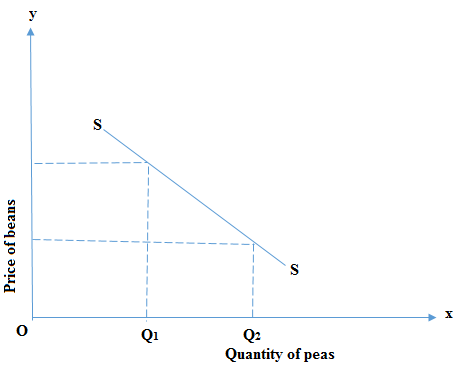
Cross Elasticity of Supply
It is the proportional (percentage) change in the supply for good x divided by the proportional (percentage) change in the price of good y.
Where:
X = Demand of good x
PY = Price of good Y
Δx = Change in demand for x
ΔPY = Change in price of Y
- CES = +ve
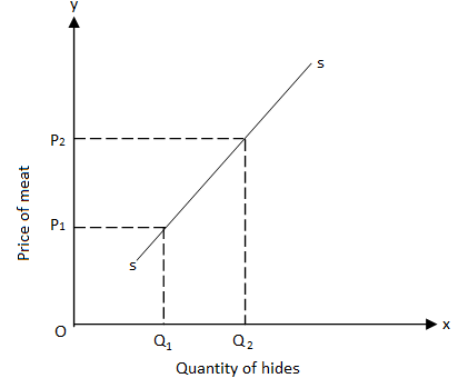
This means that the commodities in consideration are complements (jointly supplied) e.g., meat & hides. When the price of one increases, quantity supplied of the other also increases and vice versa.
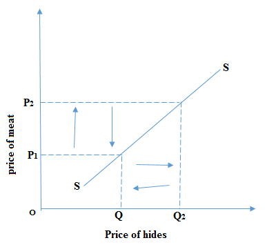
- CES = -ve
This means that the commodities in consideration are substitutes e.g., beans & peas. When the price of one increases, quantity supplied of the other decreases and vice versa.
- CES = 0
This means that the commodities in consideration are not related at all; therefore, change in price of one causes no effect in quantity supplied of the other e.g., a car and a table.
Factors of Elasticity of Supply
- Nature of commodity
Those commodities which are durable can be kept for a long time and such commodities like wheat and cloth have a greater elasticity of supply. The commodities which are perishable in nature like fish and milk have less elastic supply.
- Costs of Production
The commodities which have high costs of production have less elastic supply and vice versa.
- Those commodities which are produced in a short period of time have greater elasticity and vice versa.
- Methods of production
The commodities which can be produced with the help of simple methods of production have more elasticity and if the method of production is complicated, supply will be less elastic.
- Laws of Returns
The commodities which are produced under the conditions of increasing returns have greater elasticity of supply and the commodities which are produced under the condition of diminishing returns have smaller elasticity of supply.
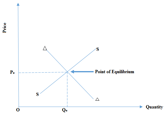
The equilibrium between Demand and Supply
- This is when quantity demanded is equal to quantity supplied; therefore, there is neither shortage nor surplus. When the demand and supply curve meet at that particular point, quantity dd is equal to quantity ss.
- The point of intersection is the equilibrium point, consisting of the equilibrium quantity and price.
| Px | Dx | Sx |
|---|---|---|
| 1 | 500 | 100 |
| 2 | 400 | 200 |
| 3 | 300 | 300 |
| 4 | 200 | 400 |
| 5 | 100 | 500 |
Price 3 is the equilibrium price and quantity 300 is the equilibrium quantity.
- The price above the equilibrium price supply increases but demand decreases and hence a surplus.
- The price below the equilibrium price, supply decreases but demand increases and hence a shortage.
The effect of changes in demand on equilibrium point, price and quantity
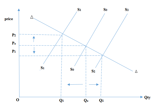
The effect of change in supply on equilibrium point, price & quantity
Demand and supply functions
- The demand function is a mathematical relationship between demand and factors that determine demand.
Qd = f(Px, TP, Y, Pr, …………)
Whereby,
Px = Price of the commodity
TP = Taste and preference
Y = Income level of consumers
Pr = Price of related goods.
Since price is the major factor that affects demand, the demand function can as well be shown using the price quantity relationship as below:
Qd = f(P)
- The supply function is a mathematical relationship between supply and the determinants of supply.
Qs = f(Px, T, NP, Pr, GP, ……………)
Whereby,
Px = Price of the commodity
T = Time
NP = Number of Producers
Pr = Price of related commodities
GP = Gestation Period
Since price is the major factor that affects supply, the supply function can as well be given as
Qns = f(P)
WAYS OF PRICE DETERMINATION
- Price mechanism
Under this, the price of the market is determined by the free interaction of the forces of demand and supply and hence determined at the point where the demand and supply curve intersect or meet.
- Sale Auction
The price is determined through bidding; therefore, it is determined by the highest bidder.
- Haggling
This is through bargaining.
- Resale price mechanism
Under this, the price of the product is determined by the producer.
- The price can as well be determined by the government and this can either be a maximum or minimum price.
Price ceiling (maximum price) is the price which is set by the government below the equilibrium price. This is normally done during the period of shortage, when price of essential goods are excessively high. Therefore, it aims at protecting consumers against such excessively high price.
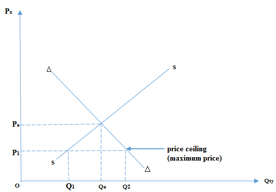
Effects of Price ceiling
- Demand will increase hence a shortage (Q1 – Q2)
- Supply will decrease
- Black market – sellers are going to sell products in order to create an artificial shortage
- Corruption & favoritism – they will sell the product to those who are willing to buy.
Advantages of price ceiling
- It helps to control inflation.
- It reduces exploitation on the consumers.
- It allows consumers to easily access essential goods at affordable prices during periods of shortage.
- It helps the government to win more support.
Disadvantages of Price Ceiling
- Discourages producers.
- It is expensive to administer.
- It creates black market.


5 Comments